Table of Contents
MA20223 2019-20' diary
Week 1
Lecture 1 (4 Feb 2020)
- Introductions and preliminaries (course structure; problem sets; hand-ins)
- Why are you here and why should you take this course?
- A mathematical model of transport
- A review of multivariable calculus (Chap. 2)
We derived the transport equation; we reviewed the visualisation of scalar and vector-valued functions.
Lecture 2 (6 Feb 2020)
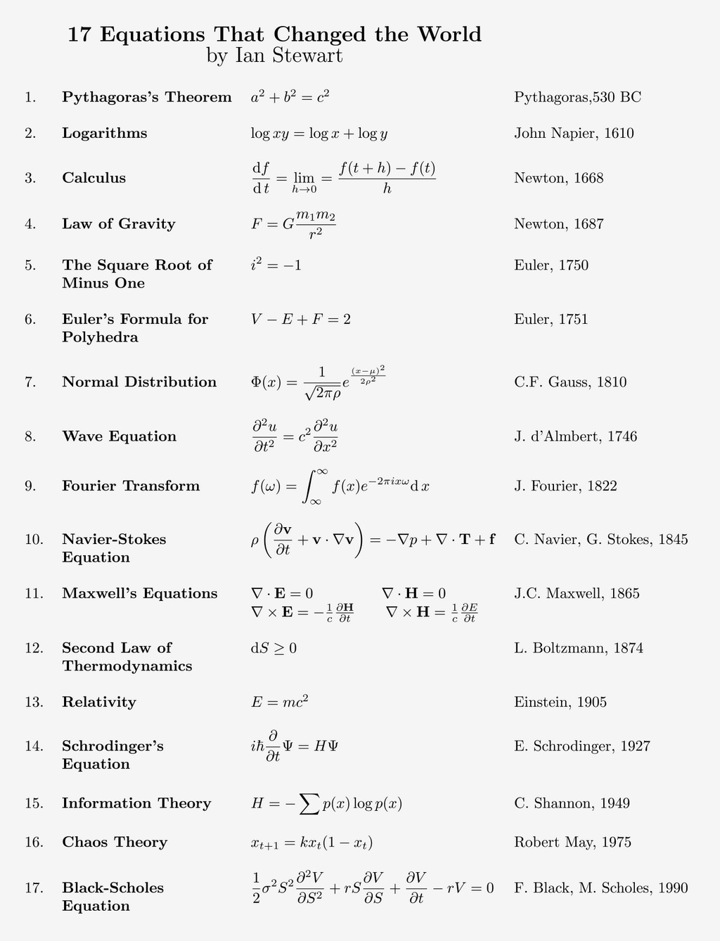
- A look at Ian Stewart's 17 equations that changed the world
- Continued review of multivariable calculus (Chap. 2)
- Line integrals (Chap. 3)
We reviewed key notions of Riemann integration (the idea of adding up infinitesimal elements), then started investigating the notion of a scalar line integral.
Lecture 3 (7 Feb 2020)
- A continued look at Chapter 3 (line integrals)
We covered the computation of scalar integrals and work integrals, doing examples for both. We also covered various properties of curves (reversability, for instance) and wrote down properties of line integrals that will be attempted as part of the homework.
Week 2
Lecture 4 (11 Feb 2020)
- Announcements: (i) typo on the PS1 with the ellipse; (ii) drop-in sessions announced.
- Chap 2: definition of conservative fields
- Chap 4: link of conservative fields and work integrals
We discussed the definition of conservative fields, and covered the important (BIG) theorem on conservative forces, and discussed its importance in the computation of work integrals. We ended with a result linking work integrals with change in kinetic energy (to be completed in lecture 5).
Lecture 5 (13 Feb 2020)
- Chap 4: Finishing up the result on work integrals and kinetic energy
- Chap 5: Parameterisation of surfaces
We discussed how surfaces can be parameterised, either via explicit, implicit, or parameteric representations. We discussed equations of planes and normals, and finally the computation of normals to surfaces.
Lecture 6 (14 Feb 2020)
- Chap 5: Finished the proof to the final Lemma about normals to surfaces
- Chap 6: Stated the two main results (flux integral and surface integral)
We discussed how to interpret surface integrals, and how to calculate the two main surface integrals (a scalar one and a vector one). This involved writing dS as a cross product. We did an example with a sphere.
Week 3
Lecture 7 (18 Feb 2020)
- A short statement and discussion about the strikes. See the Owen Jones' article "Market economics have driven universities into crisis -- and we're all paying the price"
- Explanation of the surface integral formula
- Thinking about flux integrals and their interpretation (see YouTube video)
- Chap. 7: Divergence and curl
Lecture 8 (20 Feb 2020)
- Finishing up the curl and divergence
- Doing more examples on (i) the computation of surfaces and normals; (ii) the computation of flux integrals
Lecture 9 (21 Feb 2020)
- Continued examples on (i) the computation of surfaces and normals; (ii) the computation of flux integrals
Week 4
Lecture 10 (25 Feb 2020)
- We looked at the motivation of the divergence theorem (flux through a little cuboid)
- We stated the divergence theorem
- We did examples on computations using the divergence theorem
Lecture 11 (27 Feb 2020)
- Using the divergence theorem, we proved two versions of Green's theorem
- We did examples on computations using Green's theorem (finding area)
Lecture 12 (28 Feb 2020)
- This was a complete problem set class, doing different examples of Green's theorem and the divergence theorem.
Week 5
Lecture 13 (3 Mar 2020)
- We finished off the Vector Calculus portion of the term by discussing Stokes' theorem.
- We showed the intuition of Stokes' theorem by showing the curl around a little cuboid (notice that you should read over the proof of Stokes' theorem in the typed notes).
- We did some examples on computations using Stokes' theorem
Lecture 14 (5 Mar 2020)
- We played a video by Feynmann discussing the difficulty of defining magnetism (this is a precursor to help you understand the difficulty of modelling the real world!)
- We showed off a simulation of a 2D heat equation
- We derived the heat equation in 1D.
- We began a derivation of the wave equation in 1D.
Lecture 15 (6 Mar 2020)
- We completed the derivation of the wave equation in 1D.
- We showed off a simulation of a 2D wave equation
- We used separation of variables to introduce the topic of Fourier series.
Week 6
Lecture 15 (10 Mar 2020)
- We began our investigation of Fourier series, starting off by defining terminology of periodic, even, and odd functions.
- We stated the orthogonality property of sines and cosines
Lecture 16 (12 Mar 2020)
- We derived the Fourier sine and cosine coefficients
- We defined the notion of a Fourier sine series or a Fourier cosine series
- We studied an example of estimating abs(x) using a Fourier series
Lecture 17 (13 Mar 2020)
- We did two examples of computing Fourier series