Table of Contents
Reaction-Diffusion Equations
In this chapter, we study a class of partial differential equations (PDE's) called Reaction-Diffusion Equations, which are frequently used in modeling, and describe the diffusion (spreading out) and reaction of one or several chemical species.
In the simplest one-dimensional case, let $u(x,t)$ be the concentration of some chemical positioned on the real line on $x$ at time $t$. Then, the reaction-diffusion equation has the form: \begin{equation} \frac{\partial u}{\partial t} = \underbrace{D_u \frac{\partial^2 u} {\partial x^2}}_{\text{Diffusion}} + \overbrace{f(u)}^{\text{Reaction}}, \label{eqn:reactdiffuse1D} \end{equation} where $D_u$ is a coefficient associated with the diffusive properties of $u$, and $f(u)$ is a function that describes how $u$ grows or decays depending on its current state.
If you have never come across this class of equations before, you might be wondering where they come from.
Our next task is to discuss what roles the reactive or diffusive terms play, and why we might need to combine them to achieve the desired effects.
Reactions
When you think of a “reaction”, the first image that comes to mind is probably that of a mad scientist mixing two chemicals together and causing a mild explosion. But in the case of Equation \eqref{eqn:reactdiffuse1D}, what is the lone chemical (whose concentration is $u$) reacting with? In some sense, a one-dimensional reaction means that the chemical is reacting with zero and is either making more of itself or decaying. A simple example of a decaying $f$ is \[ f(u) = -u, \] and leads to formulate the well-known model of \begin{equation} \label{eqn:decay} \frac{du}{dt} = -u, \end{equation} which has many applications including radioactive decay, and protein degradation.
It is important to understand that “reaction” is used loosely, so it is best to think of $f(u)$ as the function that describes how the concentration of $u$ changes depending on its local value.
Reactions in 2D are perhaps more intuitive since they involve two concentrations, say, $u(x,t)$ and $v(x,t)$; some examples are:
- Chemical reactions: Imagine you have a beaker and you have two chemicals and you pour them in and they begin reacting.
- Population dynamics: We have two possibilities. In a predator-prey example, the “reaction” is that whenever the predator and prey are close enough to each other the predator will eat the prey. In a competitive system, then they will not eat each other, but due to limited resources, the two populations will die off if their population density gets too high.
An example of a reaction system
Imagine that we have an isolated ecosystem with only two species. One of them feeds on the plentiful plants in the ecosystem, and the second one eats is a predator that will eat the first species and note that the “reaction” is the predator eating its prey. An Italian mathematician Vito Volterra proposed a simple model for the predator-prey model described above [(volterra_1929)]. Letting $u$ be the prey population and $v$ be the predator population, his model was, \begin{gather} \label{eqn:volt1} \frac{\partial U}{\partial t} = a_1U - a_2UV, \\ \label{eqn:volt2} \frac{\partial V}{\partial t} = a_3UV - a_4V, \end{gather} where $a_i, i\in \{1,2,3,4\}$ are growth and decay constants.
Recall what each term of the system will do:
- $a_1 U$: The prey population will grow with rate $a_1$ (i.e. the prey will reproduce proportionally to its population)
- $-a_2UV$: The prey population will decrease when the predator eats it, with predation rate $a_2$.
- $a_3UV$: If the predators have food, then they will reproduce.
- $-a_4V$: If the predators do not have food, its population will shrink.
It is useful to work with a nondimensionalised version of the equations. Writing, \begin{equation} \label{eqn:nondimenCond} u(\tau)= \frac{a_3U(t)}{a_4},\quad v(\tau) = \frac{a_2V}{a_1}, \quad \tau = a_1 t, a = \frac{a_4}{a_1}, \end{equation}
we get, \begin{gather} \label{eqn:voltND1} \frac{\partial u}{\partial \tau} = u-uv, \\ \label{eqn:voltND2} \frac{\partial v}{\partial \tau} = a(uv-v). \end{gather}
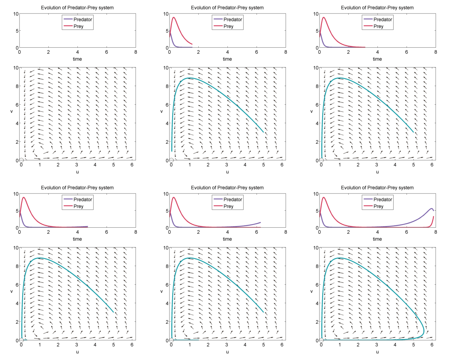
We can study the evolution of the two populations over time using a phase plane shown below. The prey population $u$ is graphed on the x-axis and the predator population $v$ is graphed on the y-axis. The arrows point in the direction of the solution to, \begin{equation} \label{eqn:phase1} \frac{dv}{du} = a\frac{uv-v}{u-uv}, \end{equation} so at a point $(u',v')$, it shows how $u(t)$ and $v(t)$ will change when the population is exactly $(u',v')$.
We can solve \eqref{eqn:phase1} exactly to get, \begin{equation} \label{eqn:closedTraj} au + v- log(u^av) = H. \end{equation} It can be shown that for $H > 1+a$, then we will get closed trajectories [(murray_2003)]. Closed trajectories tell us that the populations of u and v will change over time, but always return to their original state $(u(0),v(0))$.
Equations \eqref{eqn:voltND1} and \eqref{eqn:voltND2} have fixed points (i.e. the points where $\frac{du}{d\tau}= 0 = \frac{dv}{d\tau}$), which occur at $(0,0)$ and $(1,1)$.
When we linearise about $(0,0)$, we find that $(0,0)$is a saddle point singularity.
In addition, $(1,1)$ is neutrally stable, and the solution of the linearised equations about $(1,1)$ have the form, \begin{equation} \binom{\tilde{u}(\tau)}{\tilde{v}(\tau)} = \vec{m_1} e^{i\sqrt{a}\tau} + \vec{m_2} e^{-i\sqrt{a}\tau},\end{equation} where $\tilde{u}$ and $\tilde{v}$ are small perturbations away from $(1,1)$, and $\vec{m_1}$ and $\vec{m_2}$ are the eigenvectors. Thus, we get trajectories that look like:

Diffusion
The word diffusion comes from the Latin diffusion meaning “to pour out”. Long before it was used to describe a physical phenomenon, “diffusion” was used to describe the dissemination of knowledge, branching out, and a general abstract concept of spreading out. It was not until the 1800s that the term diffusion was used in physics to describe how particles of gases, liquids, and solids intermingle and move from areas of high concentration to low concentration without chemical combination as a result of each particle's kinetic energy. Adolf Fick described diffusion mathematically, and arrived at this result using a macroscopic approach. In fact, the diffusion equation \begin{equation} \label{eqn:FickDiffn} \frac{\partial C}{\partial t} = D \frac{\partial ^2 C}{\partial x^2}, \end{equation} is also known as Fick's second law [(mehrer_2009)].
In this set of notes, however, we will follow a microscopic derivation of the diffusion equation that is closely connected to Brownian motion.
Brownian Motion
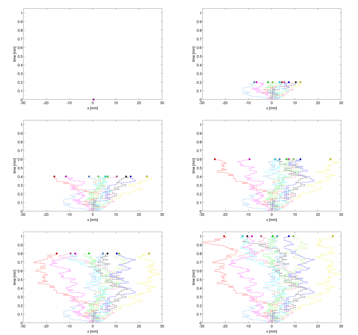
Brownian motion is named after the British botanist Robert Brown. He described “a peculiar character in the motions of the particles of pollen in water”, and more importantly he stated that this motion is not due to the particles being alive but is instead of a mechanical nature. Albert Einstein, half a century later, proposed a first approximation to Brownian motion from a physical perspective. Einstein's mental image of Brownian motion illustrates the link to diffusion. He imagined a microscopic particle (eg. one of Brown's pollen particles) suspended in liquid. The pollen particle is microscopic, but usually much larger than the molecules in the fluid, so every time it gets “hit” by the fluid molecules, the particle will move a small amount or each hit. The hits come at random intervals and from all directions [(:einstein_1956)][(nelson_1967)].
Instead of considering this 3-dimensional space, consider a 1D lattice, where, at point $x = 0, \pm h, \ldots$, we define the concentration $c(x,t)$ as the expected number of particles in position $x$ at time $t$. Let us assume first that after some time $t = t+\tau$, each particle moved right or left with equal probability $p/2$, or stayed in the same place with probability $1-p$.
Then, the expected concentration at the next point is:
\begin{equation} c(x, t+\tau) = \frac{p}{2} c(x-h, t) + \frac{p}{2} c(x+h, t) + (1-p)c(x,t) \label{eqn:discRandWalk} \end{equation}
We now want to generalize from the random walk to 1D diffusion by taking a limit as $h \rightarrow 0$ and as $\tau \rightarrow 0$.
We subtract $c(x, t)$ from both sides to get, \begin{equation} \underbrace{c(x, t+\tau) - c(x, t)}_{\Large \approx \tau \frac{\partial c}{\partial t}} = \frac{p}{2} \underbrace{[c(x-h, t) + c(x+h, t) -2c(x,t)]}_{\Large \approx h^2\frac{\partial^2c}{\partial x^2}} \label{eqn:limRandWalk} \end{equation}
Therefore, \begin{equation}\frac{\partial c(x,t)}{\partial t} = D \frac{\partial^2 c(x,t)}{\partial x^2} \label{eqn:Diffusion} \end{equation}
where we have defined the diffusion constant to be \[ D = \frac{h^2}{2\tau} \]
To see why we use reaction-diffusion equations and some of their properties go to the next section: Reaction Diffusion II
References
[(:crick_1970» author: Crick, F. ref-author: Crick title: Diffusion in Embryogenesis journal: Nature volume: 225 year: 1970 )]
[(:einstein_1956» author: Einstein, A. ref-author: Einstein publisher: Dover Publications title : Investigations on the Theory of the Brownian Movement year : 1956 )]
[(:mehrer_2009» author: Mehrer, H. and Stolwijk, N.A. ref-author: Mehrer and Stolwijk title: Heroes and Highlights in the History of Diffusion journal: Diffusion Fundamentals volume: 11 number: 1 year: 2009 )]
[(:nelson_1967» author : Nelson, E. ref-author: Nelson publisher : Princeton University Press title : Dynamical theories of Brownian motion year : 1967 )]
[(:little_2011» author: Little, SC, Tkacik G, Kneeland TB, Wiechaus EF, Gregor T ref-author: Little et al title: The Formation of the Bicoid Morphogen Gradient Requires Movement from Anteriorly Localized mRNA journal: PLoS Biology volume: 9 number: 3 year: 2011 )]
[(:kierstead_1953» author: Kierstead, H, and Slobodkin LB. ref-author: Kierstead and Slobodkin title: The size of water masses containing plankton blooms journal: J. Mar. Res volume: 12 number: 1 year: 1953 )]
[(:volterra_1929» author: Volterra V. ref-author: Volterra title: Variazioni e fluttuazioni del numero d'individui in specie animali conviventi journal: Mem. Acad. Lincei volume: 2 year: 1926 )]
[(:murray_2003» author: Murray, J.D. ref-author: Murray title: Mathematical Biology II: Spatial Models and Biomedical Applications edition: Third Edition year: 2003 publisher: Springer )]

